

In the second round, I wanted to do a medium-sized, more complicated system. The original plan was to run the Li2FeSiO4 supercell with spin polarization, which I have run extensively in VASP before. It is a nontrivial example from my previous research, and it can be tricky to get fast convergence to the right ground state. Unfortunately, I failed at getting the Li2FeSiO4 system to run. PWscf kept crashing, despite much tinkering, and all I got was the following error message:
Error in routine rdiaghg (1539): S matrix not positive definite
The QE documentation does mention these kinds of errors saying that they are related to negative charges densities in the cores, which is basically either due to an unreasonable crystal structure or a poor choice of pseudopotentials. Standard tricks like increasing the encutrho parameter or changing the diagonalization algorithm did not help either, so my guess is that something was wrong with the available PAW datasets. The all-electron Li PAW, for example, comes with a suggested plane wave cutoff of 1100 eV, unlike 272 eV in VASP. I am not sure if it is numerically sane to mix it with the other ones with much lower cutoff. I have seen this give rise to numerical instabilities in VASP, for example.
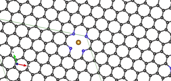
New test case: Fe-N-doped graphene
Instead, I constructed a 128-atom supercell of graphene. I inserted an Fe cation site coordinated by four pyridinic sites, to make it a little bit more exciting and also have a reason to do spin polarization.
The PAW datasets were:
Fe.pbe-spn-kjpaw_psl.0.2.1.UPF (16 valence)
C.pbe-n-kjpaw_psl.0.1.UPF (4 valence)
N.pbe-n-kjpaw_psl.0.1.UPF (5 valence)
In total, this system has 127 atoms and 524 electrons, so 512 bands per spin channel is a nice and even number here. There is a similar issue with plane-wave cutoff as in the previous example. I set it to 500 eV to compare with the VASP calculation. It could be argued that it is artificially low, and that a real production calculation with QE using the PAW potentials would need to have a bigger cutoff.
A 500 eV basis requires an FFT grid of 144x144x72 points, which in the case of VASP means that an optimal plan-wise decomposition of the FFTs can be achieved for 1,2,4,8, and 12 compute nodes by using NPAR=1,2,4,8,12, respectively. If I understand the PWscf documentation correctly, 72 FFT planes in Z-direction means that we should be able to scale up to 2x72 MPI ranks, since we have spin polarization (2 “effective” k-points), and that we are also likely to be helped by FFT task group parallelization using the -ntg command line flag.
I ran the jobs on 1,2,4,8,12, and 16 Triolith compute nodes, using all available cores (16 cores per node). For VASP, the optimal setting is band parallelization using NPAR=compute nodes, and LPLANE=.TRUE.. All PWscf calculations were run with -npool 2, which activates k-point parallelization, together with several combinations of -ntg and -ndiag, which controls FFT task parallelization and SCALAPACK linear algebra parallelization. There is experimental support for band parallelization in QE (-nband flag), but it either crashed the program or ran horribly slow, so the results below are using the standard parallelization options.
Results
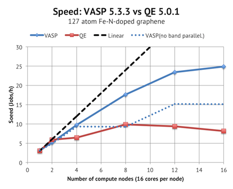
VASP scales acceptably up to 12 nodes / 192 cores, whereas QE only has decent scaling from 1 to 2 nodes. I believe that the reason is that VASP has band parallelization, but QE not. To test my theory, I ran the VASP jobs with as low NPAR as possible, which is shown as the blue dotted line. This meant NPAR=1 (no band parallelization) for 1-8 nodes, and NPAR=2 for 12-16 nodes. The parallel scaling is much worse then, and essentially flat from 8 nodes and upwards, which is similar to the QE results.
In terms of absolute performance, VASP and QE are tied again when running on 16 and 32 cores, with PWscf actually being about 10% faster on 32 cores. But when comparing the top speed, VASP achieves at least 25 Jobs/h with 16 nodes vs. 10 Jobs/h with PWscf on 8 nodes. So we are looking at half the time to solution with VASP.
Another purpose of this study was to characterize the parallelization settings for QE when running on Triolith. The best parallelization settings for this system turned out to be:
Nodes -ntg  -ndiag
1        1      16
2        1      16
4        2      16
8        2      16
12       4      16
16       4      16
FFT task groups (-ntg) seems to be necessary for higher core counts, just as suggested in the QE manual. The rule of thumb in the manual is to enable -ntg when the number of cores exceeds the number of FFT mesh points in the z direction, which seems accurate in this case.
I found the performance curve for SCALAPACK parallelization very flat for ndiag=16/25/36, so I was unable to resolve any difference with just 3-5 samples per point, but it seems like the performance flattens out above 16 cores for this system. Diagonalizing a 512x512 matrix is not that big of a task in the context of SCALAPACK, so this is not surprising.
Mixing and SCF stability turned out to be an influential factor when making the comparison between VASP and PWscf. The default mixing scheme in VASP is very good and can converge the graphene system studied here in ca 32 SCF iterations using default settings, but getting down to that level with PWscf required tuning of beta (0.2) and change of the mixing mode from plain to local-TF.
Conclusion
When it comes to bigger, more realistic calculations, PWscf is not as straightforward to work with as VASP. This is a combination of the robustness and availability of PAW datasets, and the increased need of parameter tuning necessary to get decent performance. The speed is on par with VASP for 1-2 compute nodes, but VASP has a much faster and more predictable parallel scaling beyond that. It was a surprise to me to not find working band parallelization in PWscf.